 James Dunkerley
Introduction
Enso is a functional programming language that lets you quickly and simply load, blend, and analyze your data. We’ve been building out the core capabilities of the product and are rapidly working on the IDE and cloud release to give a straightforward experience for users using it.
To show some of the new capabilities, I have tackled the first three challenges of 2023 posted on Preppin Data. These data challenges are posted by Carl Allchin, Jonathan Allenby, Jenny Martin, and Tom Prowse. They are solvable in many data tools and make an excellent set of tasks to show how to use Enso.
This blog was written using a recent nightly build; many features and functions are still maturing and subject to change as we approach our release. In addition, we are still working on adding more “widgets” to the nodes and improving data visualization capabilities to help guide you through building the workflow. These will appear over the next month or two in the nightly builds.
Week 1 — The Data Source Bank
https://preppindata.blogspot.com/2023/01/2023-week-1-data-source-bank.html
Loading a dataset into Enso is as simple as dragging the file onto the IDE, and
it will then set up the first node and attempt to parse the data. However,
Enso’s default CSV parsing only recognizes dates in ISO format (yyyy-MM-dd).
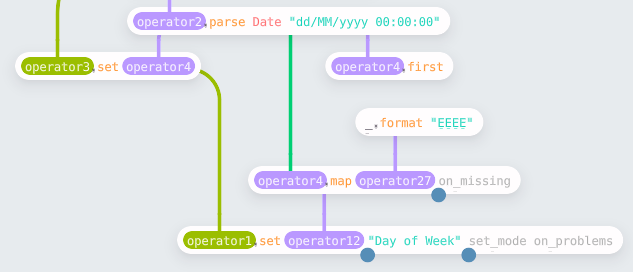
So to parse the ‘Transaction Date’ column, we need to select it (using the get
method) and then parse it (using the parse method), and finally replace the
original column in the table (with the set method).
For this challenge, we need to derive three values — the day of the week, the bank code, and whether a transaction was in-person or online. For the first two, I used the same process — select the column, apply a function over each row, and then add the result to the table.
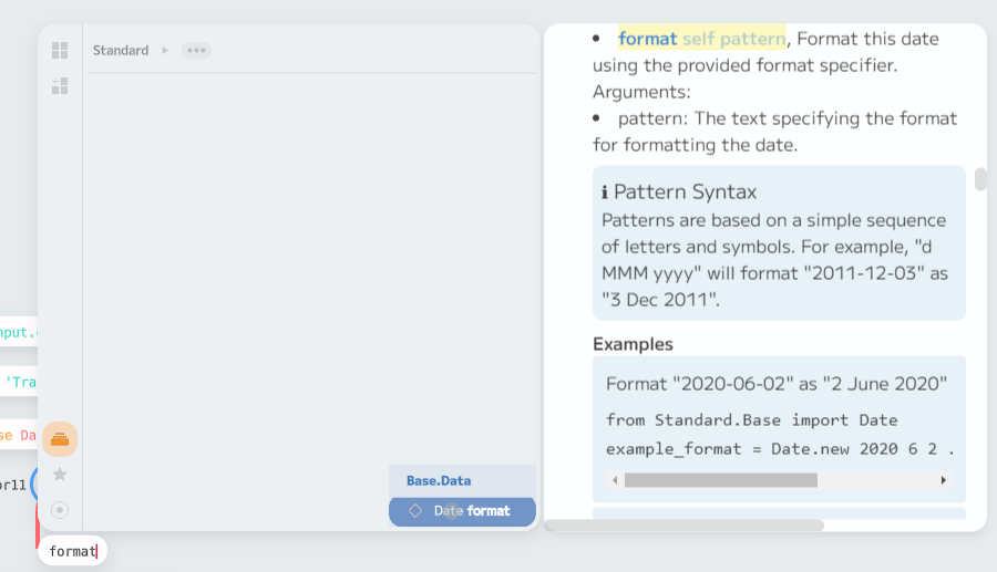
Creating the “day of week” column involves formatting the date. The format
function on a Date allows for this. Enso uses Java for date and times, so the
usual date format specifiers
work — so in this case, the expression is _.format “EEEE” (the _ is a
shorthand to create a lambda function). To build this within the IDE, I took a
single value from the column (using .first), and then the component browser
showed the available functions for a Date. If you then detach the incoming
node, the new node becomes a reusable function I can feed into the map
function on the column.
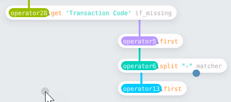
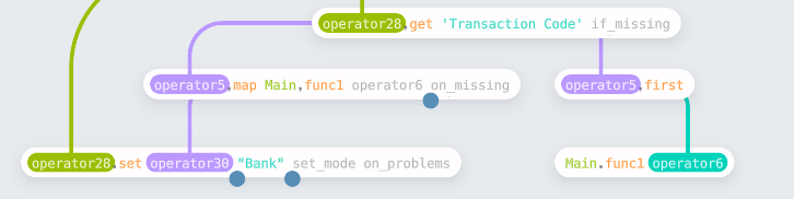
For the “bank” column, we need to split the “Transaction Code” string and take
the first part. The process was the same — pick the input column, get a single
value, and create a mapping function. In this case, the mapping used the split
and first functions.
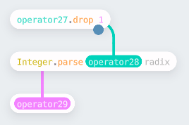
Having built these nodes, Enso allows me to make a reusable function by
selecting them and pressing Ctrl-G. The result can then be
fed into the same map as above.
The final column was created using Enso expressions, an Excel formula-like
syntax allowing a shorthand to derive a new column. You can reference existing
columns (specified by name in square brackets) and use all the functionality
defined on a column. In this case,
‘IF [Online or In-Person]==2 then “In-Person” else “Online”’ will decode the
column into the text values.
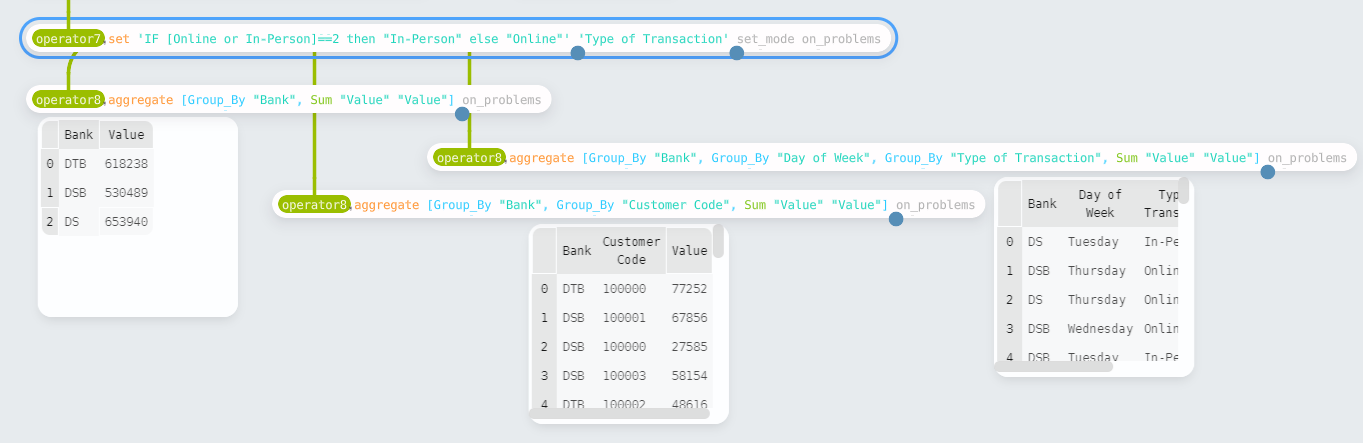
Finally, the last task is aggregating the results to produce the three new
tables. The aggregate function allows us to do this. It takes a vector of
Aggregate_Column to create the summarized tables. These columns are either
group bys or aggregate calculations. For example,
operator8.aggregate [Group_By “Bank”, Group_By “Day of Week”, Group_By “Type of Transaction”, Sum “Value” “Value”].
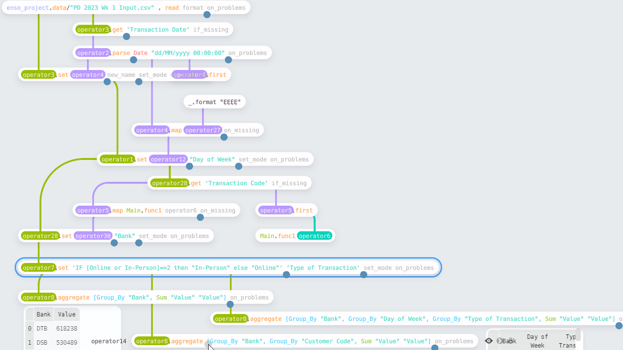
The final workflow is shown below:
Week 2 — International Bank Account Numbers
https://preppindata.blogspot.com/2023/01/2023-week-2-international-bank-account.html
For the second challenge, we need to construct “IBAN” codes for a set of
transactions. In this case, two input files are provided — one with SWIFT codes
for banks and another with transaction data. There is one slight complication
with bringing the data in. All the values are text in the “Swift Codes” file, so
Enso doesn’t automatically detect the headers. The use_first_row_as_names
function renames the columns to the first value.
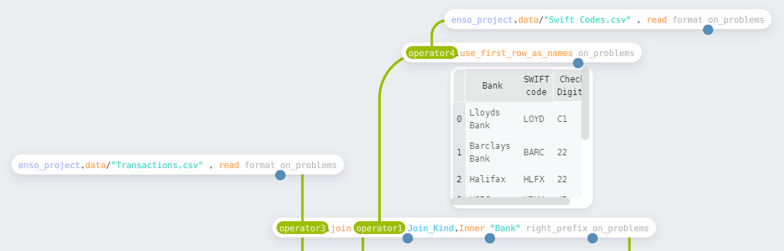
Having read the files, the next step is to join the two data sets. The join
function allows you to specify the type of join (such as Inner, Left_Outer,
Full) and the columns to join on (defined as a Vector). For this function,
if the two inputs have the same first column, it will, by default, automatically
perform an inner join using this.
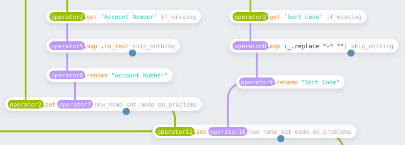
There is a small amount of preparation before creating the IBAN for each
transaction. First, the transaction file has been automatically parsed, and the
account numbers have been converted to integers. However, to concatenate these
values in the final expression, they must be converted back to text. Using the
same process as week 1 to create a derived value, the map function uses
.to_text to convert the values. For the “Sort Code,” we need to remove -
from the values; a simple replace on each record covers this.
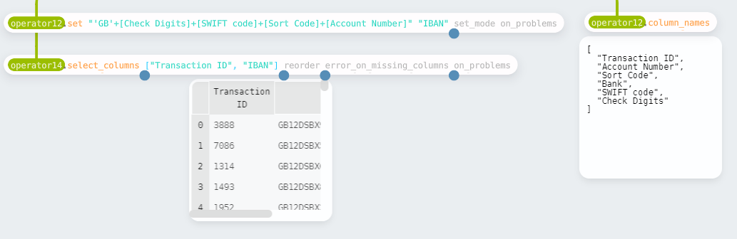
The final step is to concatenate the various parts of the IBAN into a single value. I chose to use the expression syntax again here.
The final workflow is shown below:

Week 3 — Targets for DSB
https://preppindata.blogspot.com/2023/01/2023-week-3-targets-for-dsb.html
For the final challenge in this post, the task is to compare the actual quarterly revenue of DSB against some provided targets. This task builds on top of the work of week 1. The first step is to get the quarterly totals.
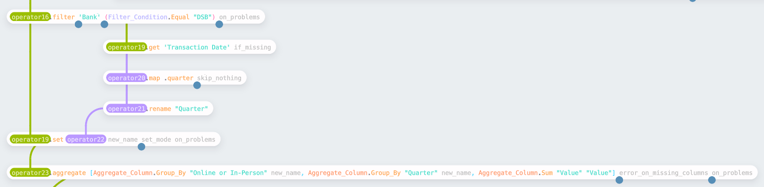
Starting from the pre-aggregated table in week 1, the data is filtered down to
just the transactions for DSB. The filter node allows you to specify various
ways to filter the data, such as a simple equality check. You can also use
filter_by_expression using the expression syntax if preferred (for this case,
it would be [Bank] == ‘DSB’). Having filtered the data, the quarter for the
dates is added as a new column and then aggregated into the summary table.
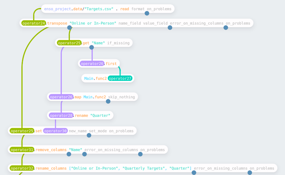
The next task is to read in and reformat the input file containing the targets.
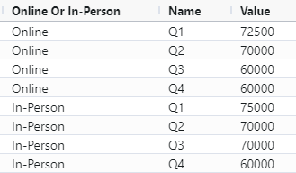
This file is in a column-based format; we want to convert this to rows. The
transpose function allows us to do this — the first argument is one or more
columns to leave unchanged and keep as id fields; the other columns will be
transposed into a Name and Value column.
To join these targets to the aggregated data, the “Name” column must be
parsed, first removing a “Q” and then converting to an integer.
This follows the standard pattern of picking a column, creating a reusable
function (as shown above), apply to each row using a map, and writing back into
the table. Finally, remove the “Name” column and rename the remaining columns
to create the tidied targets to join the totals.
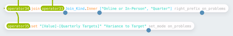
This join requires two fields to be equal — as the names match, these can be
specified as a vector of strings. More complicated join conditions can be used
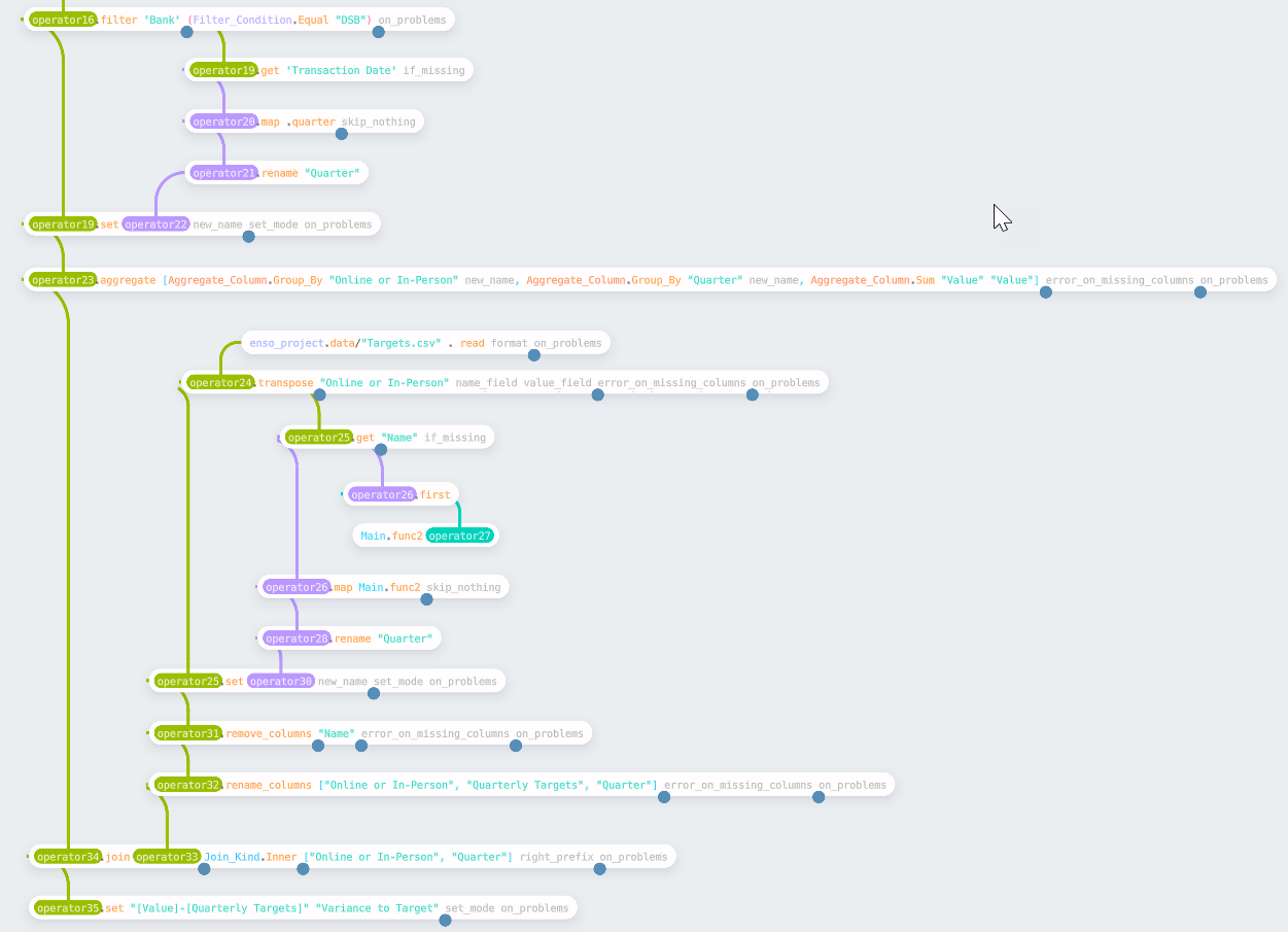
by using the Join_Condition type. Finally, the last step is to compute the
variances — this time using the expression syntax.
The final workflow (built on top of part 1) is shown below:
Summary
Hopefully, these examples give you a feel of how to use Enso. If you want to try it, download a nightly release from our GitHub or look for the forthcoming beta release in a few months.