
 James Dunkerley
Introduction
In this post, I will build on top of my last post and go over how to parse values in the dataset, select down to just the columns we are interested in, and finally aggregate the data. The previous post covered installing Enso and then loading in some data.
This post starts from the workflow created in the last post, still using the Kaggle Superstore Dataset. If you have not read that post, I recommend you do so before continuing. That workflow can be downloaded from here.
The goal of this workflow will be to get a table of the total sales by category for each month (using the order date).
Parsing the Data
Let’s start by taking a look at the structure of the data. We can do this using
the info function on the first node. To add this node, select the first node
and press Return or drag out from the bottom of the first node. Then,
in the new node, type info or choose it from the Component Browser. This
function returns a new table containing the metadata about the table. In this
case:
| Column | Items Count | Value Type |
|---|---|---|
| Row ID | 9994 | Integer (64 bits) |
| Order ID | 9994 | Char (variable length, max_size=unlimited) |
| Order Date | 9994 | Char (variable length, max_size=unlimited) |
| Ship Date | 9994 | Char (variable length, max_size=unlimited) |
| Ship Mode | 9994 | Char (variable length, max_size=unlimited) |
| Customer ID | 9994 | Char (variable length, max_size=unlimited) |
| Customer Name | 9994 | Char (variable length, max_size=unlimited) |
| Segment | 9994 | Char (variable length, max_size=unlimited) |
| Country | 9994 | Char (variable length, max_size=unlimited) |
| City | 9994 | Char (variable length, max_size=unlimited) |
| State | 9994 | Char (variable length, max_size=unlimited) |
| Postal Code | 9994 | Char (variable length, max_size=unlimited) |
| Region | 9994 | Char (variable length, max_size=unlimited) |
| Product ID | 9994 | Char (variable length, max_size=unlimited) |
| Category | 9994 | Char (variable length, max_size=unlimited) |
| Sub-Category | 9994 | Char (variable length, max_size=unlimited) |
| Product Name | 9994 | Char (variable length, max_size=unlimited) |
| Sales | 9994 | Float (64 bits) |
| Quantity | 9994 | Integer (64 bits) |
| Discount | 9994 | Float (64 bits) |
| Profit | 9994 | Float (64 bits) |
Enso will automatically parse columns of all numbers (such as Sales,
Quantity, and Profit) and recognise standard format dates and times (such as
2023-11-09 or 2023-11-09 12:22:04).
At first glance, the Postal Code column appears to be a number (US 5-digit Zip
codes), but as some have leading 0s, Enso will not parse this column by default.
While we probably would want to keep these as text values, we can convert this
to a number (specifically, an integer) using the table’s parse function.

Once we have added the node, the next step is to choose the columns we are
interested in and to specify the target type. Click on the right of the column
placeholder to add a new name, then pick Postal Code from the dropdown.
Finally, select Integer from the type dropdown.
In this dataset, the date fields are stored in US format without leading zeros. Enso uses similar format strings to .NET to specify how to parse or format dates. The table below is not an exhaustive list but gives some key date specifiers.
| Specifier | Description | Example |
|---|---|---|
| d | Day of month (1 to 31) | 1 |
| dd | Day of month (2 digit, 01 to 31) | 01 |
| ddd | Day of week (short name) | Mon |
| dddd | Day of week (full name) | Monday |
| M | Month of year (1 to 12) | 1 |
| MM | Month of year (2 digit, 01 to 12) | 01 |
| MMM | Month of year (short name) | Jan |
| MMMM | Month of year (full name) | January |
| yy | Year (2 digit) | 23 |
| yyyy | Year (4 digit) | 2023 |
The US format of M/d/yyyy is used to parse the Order Date and Ship Date
columns. Add a new parse node and two entries to the columns placeholder.
Then, choose Order Date and Ship Date from the dropdowns. Next, select
Date from the type dropdown.

At this point, the node will be surrounded by a yellow border, indicating that a
problem has occurred when trying to parse these columns. By default, Enso
attaches a warning to the resulting table and puts a Nothing value in for the
cells it cannot parse. In this case, the format of the dates has not yet been
given. There are two ways to set the format: add a new node (using the +
button) and enter the value “M/d/yyyy”, or edit the existing node and type the
value at the end of the code. To edit the node, Ctrl-click on it, and
it will switch to a text box showing the code. Type the format string at the end
of the code preceded by a space ( “M/d/yyyy”). The yellow border will
disappear, and the warning will be removed.

The new IDE (coming soon) will have significantly improved support for editing text placeholders.
The last two parameters in the parse function allow more control over the
error handling. By default, if a column you have chosen does not exist, the
function will error and stop. If you wish to allow this to continue, select
False in the error_on_missing_columns dropdown, and a warning will be
attached to the result instead of the process erroring.
The final parameter, on_problems, specifies what Enso should do with warnings.
This argument is present in a lot of our functions. Generally, warnings are
attached to the result and can be examined or handled within the workflow. You
can choose one of the following from the dropdown to control this.
Ignore: warnings are ignored, and the result is returned.Report Warning: warnings are attached to the result and then returnedReport Error: warnings are treated as a dataflow error, and the error is returned instead of the result.
In a later post, I will fully cover how to handle warnings and errors.
Selecting Columns
Order Date, Category, and Sales are the only columns needed for this task.
To choose these columns, add a new node connected to the second parse node and
choose select_columns from the component browser.
Add three new entries to the columns argument and choose the required columns
from the dropdowns under each. The select_columns function will return a new
table containing only the columns you have selected.
By default, the columns will be in the same order as the source table. Choose
True from the reorder dropdown to return the columns in the order of the
select list. The names are matched case-sensitively. To allow case differences,
choose Insensitive from the case_sensitivity dropdown.
Adding Month and Year Columns
The table now contains only the interested columns, but we need to extract the
month and year from the Order Date column. The set function allows us to
derive a value from an existing column and add it to the table. Add a new node
connected to the select_columns node and choose set from the component
browser.

The first parameter, column, defines the new column, which can be done in a
few different ways (I will cover more of these methods in a later post). For
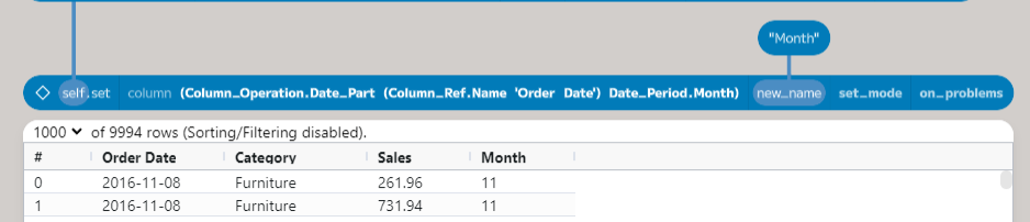
this post, we will use a Column_Operation. To add the month as a column,
choose “date part” from the dropdown and pick “Order Date” for the input and
Month from the period. A new column called date_part([Order Date], Month)
will be added. We want to rename this to “Month”. If you add a new node with a
value of ”Month” and then connect to new_name, the column will be renamed.
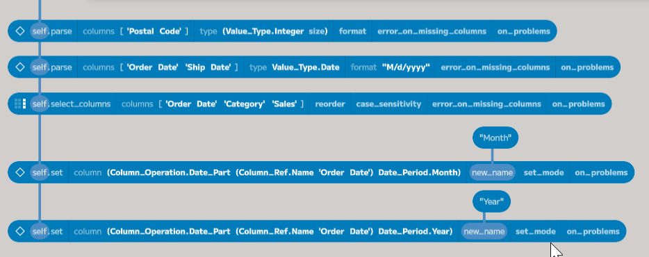
Using the same process to add a new column for the year, the table now has all the data needed to aggregate.
Grouping and Aggregating
The last step to produce the table is to aggregate the data. Add a new
aggregate node connected to the set function, which added the year. This
function takes a list of Aggregate_Columns, which define the grouping (via
Aggregate_Column.Group_By) and the method we’ve chosen for aggregation (such
as the sum of sales). In this case, we want to group by Category, Year, and
Month and then sum the Sales.

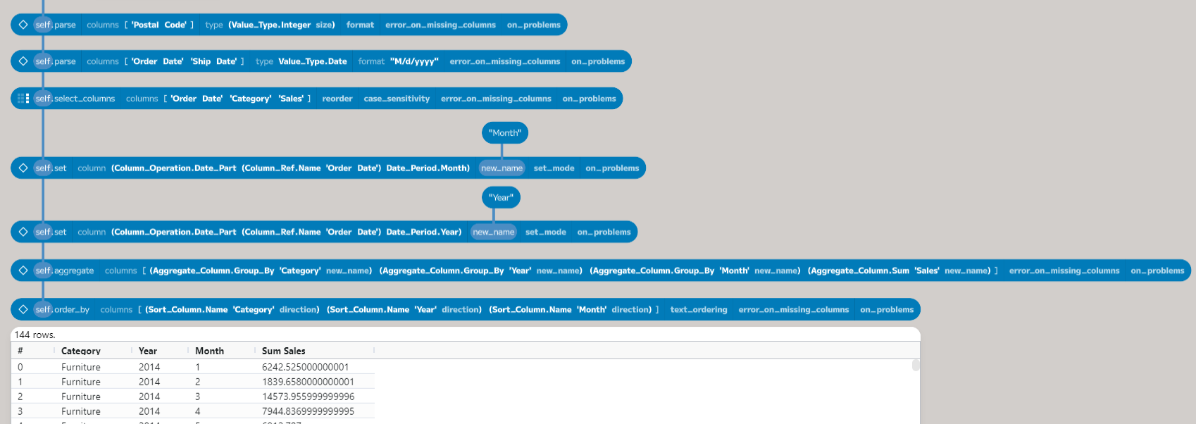
Add four entries into the columns argument and then select group by for the first three and sum for the last. Then, choose the appropriate columns from the dropdowns. The aggregate function will return a new table with the aggregated data. This function does tend to be quite verbose. Later versions of the IDE should offer a more concise view of the configured aggregate function.
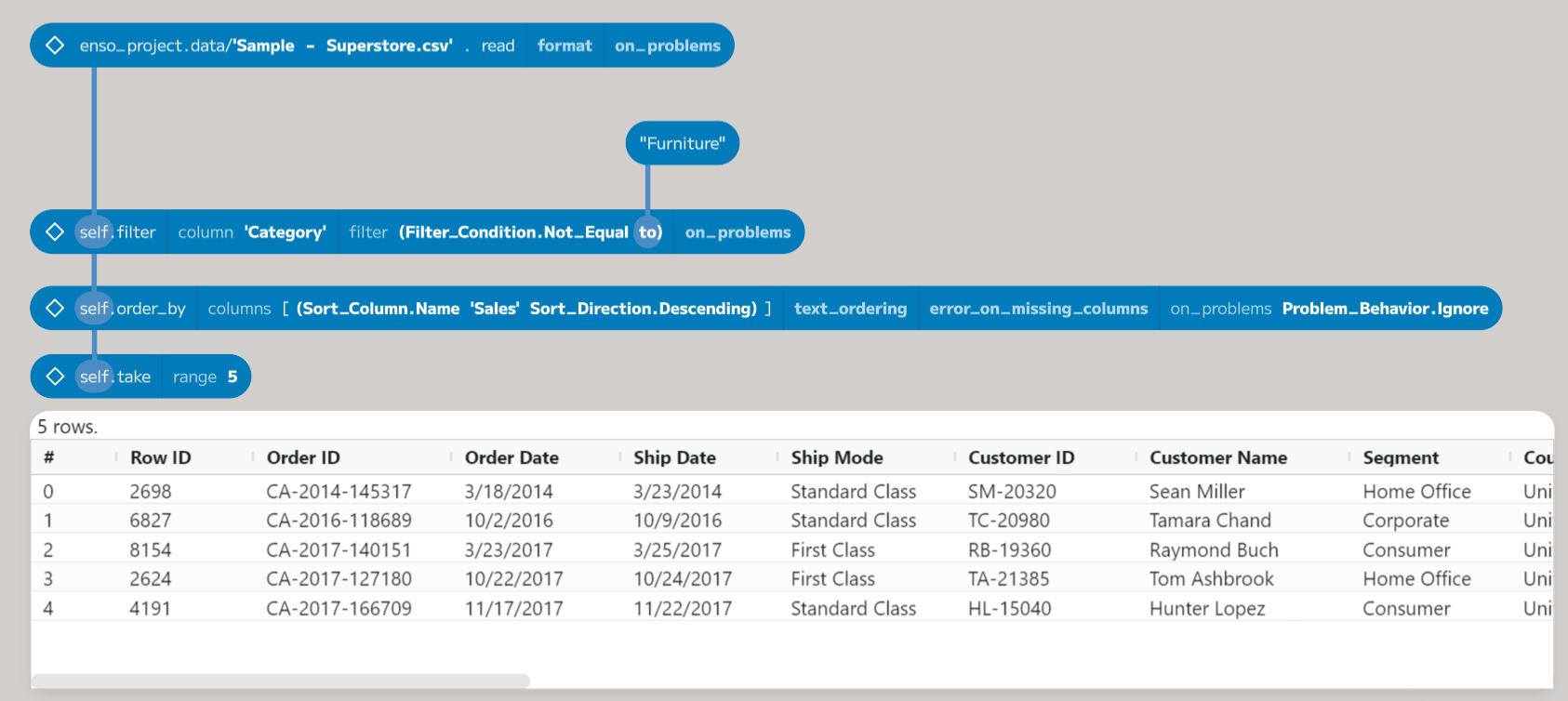
The grouped table is not returned in a specific order. To sort the data into the
required order, use the order_by function as shown in the previous post. The
completed process is shown below.
Conclusion
In this post, we have introduced a few more functions and covered some of the basics of parsing, selecting, and grouping data. So far, we have used the following functions:
filter: choosing specific rows from a table based on a condition.order_by: sorting the rows in a table.info: getting the metadata about a table.parse: converting columns to a different type.select_columns: choosing a set of columns from a table.set: adding a new column to a table.aggregate: grouping and aggregating data.
The following post in this series will cover how to join tables together.
As before, I hope you will consider trying out Enso. We are working hard to make it a fantastic product and would love your feedback. If you have any questions, please join our Discord server.